What Is a Good Sharpe Ratio | Benchmarks and Red Flags for Bots

By FullStack Alpha Editorial Team | Reviewed by Jay Rocco, Chief Editor

A good Sharpe ratio is generally anything above 1.0, which Investopedia describes as the level “generally considered good,” and for a trading bot we treat 1.0 to 2.0 on a live, cost-inclusive record as solid and anything above 3.0 as a claim to verify before you believe it. The Sharpe ratio is your average return above the risk-free rate divided by the volatility of those returns, so it measures how much you were paid for the bumps you sat through. For context, the S&P 500’s long-run Sharpe ratio on annual data from 1928 through 2025 works out to about 0.43 using NYU Stern’s historical return series. That is why a backtest showing 2.5 or more should make you suspicious, not excited: overfitting, short samples and missing costs inflate the number far more often than skill does.

Key insights

• Formula: (average return minus risk-free rate) divided by the standard deviation of returns, per William Sharpe’s own 1994 paper, where he called it “historic average differential return per unit of historic variability.”
• The S&P 500’s annual Sharpe ratio was about 0.43 for 1928 to 2025 and about 0.82 for 2015 to 2025, our calculation from Damodaran’s historical returns. Trailing 12-month figures swing far more.
• Andrew Lo found a hedge fund’s annual Sharpe ratio can be “overstated by as much as 65 percent” because of serial correlation in monthly returns.
• In our simulation, the best of 100 strategies with zero real edge showed an annualized Sharpe ratio of about 1.8 on two years of daily data. Testing many variants manufactures good-looking numbers.
• Decision rule: judge a good Sharpe ratio only on live or out-of-sample, cost-inclusive returns, next to drawdown and trade count.

What Is the Sharpe Ratio in Plain Words?

The Sharpe ratio is return above the risk-free rate, divided by volatility. It tells you how much extra reward you got for each unit of bumpiness in your returns. That is the whole idea.

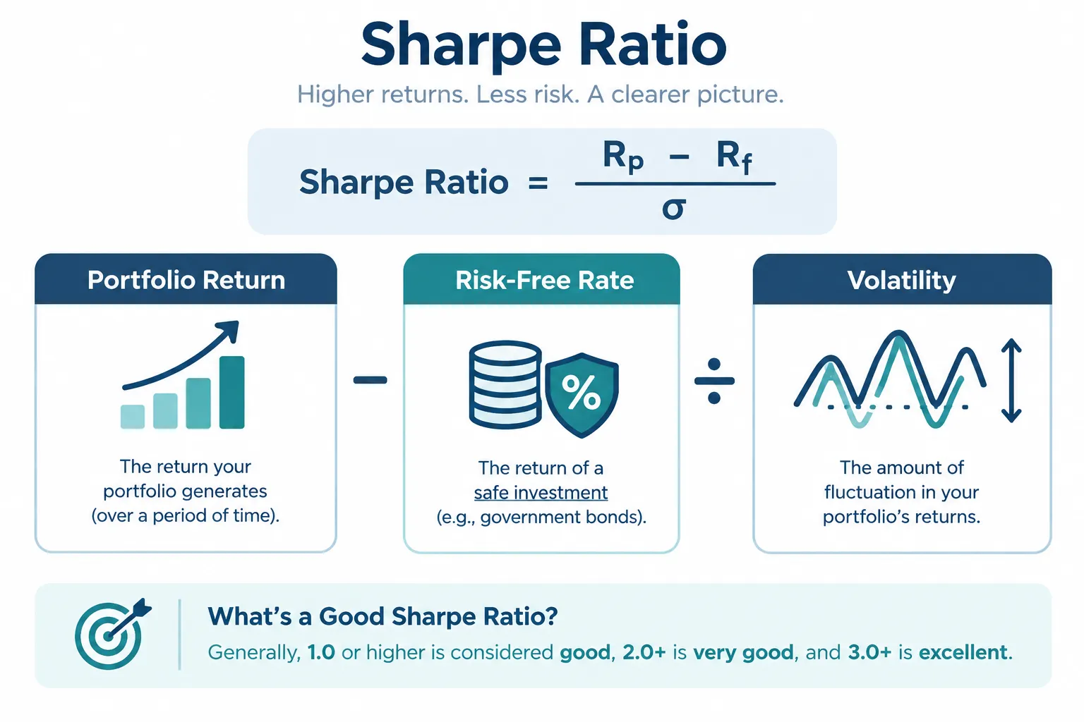
William Sharpe introduced it in 1966 as the “reward-to-variability ratio,” and the name Sharpe ratio stuck later. In his 1994 paper in The Journal of Portfolio Management, he defines the historic version as the average of the differential return (your return minus a benchmark such as Treasury bills, period by period) divided by the standard deviation of that differential return. Sharpe won the Nobel Prize in economics in 1990, per the Nobel Prize site.

A worked example. Say a trading bot averages 12% a year. Treasury bills paid 4%. That leaves 8% of excess return. The bot’s yearly returns have a standard deviation of 10%. Divide 8 by 10 and the Sharpe ratio is 0.8.

A second bot earns the same 8% excess return with a standard deviation of only 4%, because its equity curve is smoother. Divide 8 by 4 and its Sharpe ratio is 2.0. Same profit, very different ride. That is the point of the ratio: it is not about how much you made, it is about how much pain you took to make it.

Volatility here means the statistical spread of your returns over time, measured daily, weekly or monthly. A system that wins steadily and loses in small steps has low volatility. A system with an occasional blowup month has high volatility, even if its average looks fine.

The risk-free rate moves too. In Damodaran’s data, the average three-month T-bill rate was 0.04% in 2021 and 5.28% in 2023. A strategy needs about five points more raw return in a 5% T-bill world to post the same Sharpe ratio it would have posted when bills paid almost nothing. A lot of bot marketing quietly skips that detail.

Decision rule: if you cannot describe your bot’s volatility in plain terms (“it loses about X% in a bad month”), you do not really understand its Sharpe ratio. You are just quoting a number.

What Is a Good Sharpe Ratio for a Trading Bot?

A good Sharpe ratio for a trading bot is above 1.0 on a live, cost-inclusive record, with 1.0 to 2.0 the range where most real, working systems land. Below 1.0 is weak or inconclusive. Above 2.0 is strong but deserves a hard look at how it was measured. Above 3.0, assume something is off until proven otherwise.

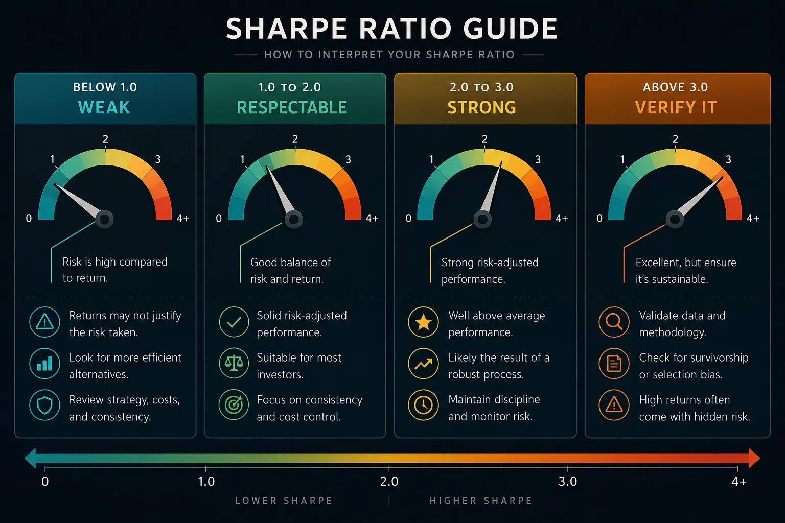
The anchor for a good Sharpe ratio is simple: Investopedia says Sharpe ratios above one “are generally considered ‘good,’” and adds that investors compare against peers, so a 1.0 can look weak if rivals sit at 1.2. The higher bands below are our own rules of thumb for bots, built on the research in the rest of this article, not a universal standard.

Sharpe Band	Common Label	What It Means for a Bot
Below 0	Losing money for the risk taken	The bot did worse than T-bills. Kill it or rebuild it.
0 to 1.0	Weak or inconclusive	Some return, not much per unit of risk. The long-run S&P 500 sits here (about 0.43 on annual data since 1928).
1.0 to 2.0	Good	A defensible system if the record is live, cost-inclusive and long enough.
2.0 to 3.0	Strong	Impressive if live. Ask for the sample length, the number of variants tested and the cost model.
Above 3.0	Verify before believing	Rare in genuine live trading. Usually overfitting, a short window, serial correlation or missing slippage.

Those bands assume a live or walk-forward record that includes fees, spreads and slippage. A backtest-only Sharpe ratio needs a heavy discount. Our piece on paper trading slippage shows how much friction disappears in simulated fills.

Decision rule: if a bot’s sales page shows a Sharpe ratio above 2.5 and does not say whether it is backtested or live, assume it is backtested and inflated. Ask for the live number before you fund anything.

Match the benchmark to the risk. A market-neutral strategy at 1.2 may be doing more real work than a leveraged directional strategy at 2.0, because the leveraged one carries tail risk the ratio does not show. Sharpe himself notes the ratio “does not take correlations into account” with what you already own.

Is a Sharpe Ratio of 0.5 Good?

No. A Sharpe ratio of 0.5 falls below the 1.0 line that marks a good Sharpe ratio, so for a bot it is weak to inconclusive. It means about half a unit of excess return per unit of volatility.

Context still matters, and the S&P 500 is the best context there is. On annual data from 1928 to 2025, the index’s Sharpe ratio was about 0.43. Buying the index and holding it for nearly a century, one of the best wealth builders in history, scored below 0.5. So a 0.5 is not a failure for a long-only stock portfolio. It is a failure for a bot charging a subscription to beat that portfolio.

Sample length decides how much a 0.5 tells you. On three months of data it means almost nothing. On five years, net of costs, it says the strategy is consistent but not worth extra risk or fees.

Common mistake: treating one quarter’s Sharpe ratio as stable. A system can show 0.5 one quarter and 1.8 the next from noise alone, with nothing about the strategy changing.

What Is the Sharpe Ratio of the S&P 500?

The S&P 500’s Sharpe ratio depends heavily on the window and the data frequency. On annual returns with dividends minus the three-month T-bill rate, it was about 0.43 from 1928 to 2025, about 0.57 from 1975 to 2025 and about 0.82 from 2015 to 2025. Trailing 12-month figures move far more: Investopedia quoted 1.72 in mid 2026, and PortfoliosLab’s trailing one-year figure was 0.94 by late 2026.

Worked example: the index’s long-run Sharpe ratio

We computed these from Aswath Damodaran’s historical returns table at NYU Stern (S&P 500 with dividends and the average three-month T-bill rate each year). For 1928 to 2025:

• Average annual S&P 500 return: 11.86%
• Average T-bill return: 3.42%
• Average excess return: 8.44%
• Standard deviation of annual excess returns: 19.70%
• Sharpe ratio: 8.44 / 19.70 = about 0.43

The same math on shorter windows:

Window	Avg excess return	Std dev	Sharpe ratio
1928 to 2025	8.44%	19.70%	0.43
1975 to 2025	9.24%	16.12%	0.57
2000 to 2025	7.63%	18.13%	0.42
2015 to 2025	12.40%	15.11%	0.82

These use simple averages of annual returns, so they will not match figures computed from monthly or daily data. That is the lesson: quote the window, the frequency and the risk-free rate, or the number is meaningless.

Decision rule: use the S&P 500 as a sanity check, not a target. If a bot claims to triple the index’s Sharpe ratio over the same window, ask for the calculation period, data frequency and risk-free rate before you believe it.

How Do You Calculate the Sharpe Ratio Step by Step?

Subtract the risk-free rate from each period’s return, average those excess returns, divide by their standard deviation, then annualize if you need to.

1. Pick a frequency. Daily, monthly or annual. Stay consistent.
2. Compute excess returns. For each period, subtract the matching risk-free rate (a T-bill yield for the same period).
3. Average the excess returns.
4. Take the standard deviation of the excess returns over the same periods.
5. Divide the average by the standard deviation. That is the Sharpe ratio for that frequency.
6. Annualize if needed. Multiply a monthly Sharpe ratio by the square root of 12, or a daily one by the square root of 252 trading days.

Worked example. A bot posts an average daily excess return of 0.08% with a daily standard deviation of 0.5%. Daily Sharpe ratio = 0.08 / 0.5 = 0.16. Annualized = 0.16 x the square root of 252 (about 15.87) = about 2.54.

That square-root step is where sloppy marketing hides. Sharpe’s own paper says the square-root-of-T scaling holds under simplifying assumptions, including no serial correlation. Andrew Lo’s 2002 study in the Financial Analysts Journal found that multiplying monthly Sharpe ratios by the square root of 12 is generally incorrect when returns are serially correlated, and that a hedge fund’s annual Sharpe ratio can be “overstated by as much as 65 percent.” A bot that trades the same setup over and over, with returns that are not independent day to day, can show an annualized number far above what the strategy earns.

Doing it in a spreadsheet

You do not need code. With monthly returns in column B and the matching monthly T-bill return in column C:

1. In column D, compute excess return: =B2-C2, filled down.
2. Monthly Sharpe ratio: =AVERAGE(D2:D61)/STDEV.S(D2:D61) for five years of months.
3. Annualized: multiply the result by SQRT(12).
4. Autocorrelation check: =CORREL(D2:D60,D3:D61). If it is clearly positive, the annualized figure is likely overstated, per Lo.

Use the sample standard deviation (STDEV.S), and use the same months for every column. If your broker exports daily equity instead of returns, convert to monthly returns first, so a single noisy day does not dominate the result.

Common mistake: annualizing a short, high-frequency sample without checking autocorrelation. If returns on consecutive days are correlated, treat the annualized number as optimistic.

How Long a Track Record Does a Good Sharpe Ratio Need?

A good Sharpe ratio needs years, not months, before it means much. The estimate itself is noisy, and the noise shrinks only with the square root of time.

Worked example: a real 1.0 strategy, measured over different windows

We simulated a strategy with a true annualized Sharpe ratio of exactly 1.0 (daily returns, normally distributed, no autocorrelation) and measured it over different lengths of history, 20,000 times each:

Track record	Spread of the measured Sharpe (std dev)	Chance it shows 0 or below	Bottom 5% of measured Sharpe
1 year	about 1.00	about 16%	about -0.65
2 years	about 0.71	about 8%	about -0.16
4 years	about 0.50	about 2%	about 0.18
8 years	about 0.35	about 0.2%	about 0.43

Read the first row slowly. A genuinely good strategy, measured over one year, shows a Sharpe ratio of zero or worse about one time in six. Flip it around and the same noise means a strategy with no edge can easily show 1.0 or more over a year.

The pattern follows a simple rule of thumb under these idealized assumptions: the spread of an annualized Sharpe estimate is roughly 1 divided by the square root of the number of years. Real returns, with fat tails and autocorrelation, are noisier still, which is exactly what Lo’s study and the Deflated Sharpe Ratio account for.

Decision rule: for a claimed Sharpe ratio of about 1.0, ask for at least four years of live or truly out-of-sample results before treating it as real. For a short record, look at the number of trades and the drawdown instead, because the Sharpe ratio will not settle down in time to help you.

Why Does a Sharpe Ratio of 2.3 From an AI Backtest Need a Second Look?

A Sharpe ratio of 2.3 from an AI backtest needs a second look because backtests are easy to over-optimize, and the more variants you try, the better the best one looks by luck alone. A good Sharpe ratio from a backtest is a starting point for questions, not an answer. The number is not the problem. The process behind it usually is.

Worked example: how luck manufactures a 1.8

We ran a simple simulation. Each “strategy” was 504 trading days (two years) of random daily returns with a true average of exactly zero: no edge at all. We annualized each one’s Sharpe ratio and kept the best of the batch, and repeated that thousands of times.

Strategies tested	Average best Sharpe ratio (zero true edge)
10	about 1.1
100	about 1.8
1,000	about 2.3

The spread of a single zero-edge strategy’s two-year Sharpe ratio was about 0.71, and about 8% of them scored above 1.0 by chance. Test 1,000 parameter combinations, the kind of sweep an AI coding assistant can run in an afternoon, and the winner shows a 2.3 with nothing behind it.

That is the problem the Deflated Sharpe Ratio (Bailey and López de Prado, The Journal of Portfolio Management, 2014) was built to fix. It adjusts a Sharpe ratio for the number of trials, the sample length and non-normal returns (skew and fat tails), and estimates the probability the result reflects skill rather than selection. A related framework, the Probability of Backtest Overfitting by Bailey, Borwein, López de Prado and Zhu (Journal of Computational Finance, 2017), uses combinatorially symmetric cross-validation to estimate how likely the best in-sample strategy is to underperform out of sample.

Checklist before you trust a 2.3:

• How many variants were tested? If the answer is “lots” or “the AI optimized it,” discount hard.
• Trading costs. Does it include commissions, spreads and slippage at realistic sizes?
• Sample length. Six months or six years?
• Look-ahead bias. Did the code use information not available at trade time? Our look-ahead bias guide shows how AI-written backtests leak future data.
• Out-of-sample test. Did the 2.3 hold on data the model never touched during development?

Decision rule: if a vendor shows a Sharpe ratio above 2.0 without separating backtest from live, stating the sample window or saying how many variants were tried, treat it as marketing. Our list of AI trading bot red flags covers the other tells.

Sortino vs Sharpe, Which Should Bot Builders Use?

The Sortino ratio penalizes only downside volatility, while the Sharpe ratio penalizes upside and downside swings equally. For a bot with lots of small wins and occasional big wins, Sortino often paints a fairer picture. For a bot with hidden crash risk, neither ratio alone protects you.

Investopedia describes the Sortino ratio as a Sharpe variation that “ignores above-average returns to focus solely on downside deviation.” A related cousin, the Treynor ratio, divides excess return by beta instead of total volatility.

Feature	Sharpe Ratio	Sortino Ratio
What it penalizes	All volatility, up and down	Only downside deviation below a target
Best suited for	Roughly symmetric returns	Strategies with frequent small gains and occasional spikes
Weakness	Punishes good upside swings the same as bad ones	Can look great while hiding fat-tail crash risk
Red flag it misses	Negative skew, rare severe losses	Same blind spot, often worse because the downside sample is small

Here is the danger for bot builders. A short-volatility strategy, a grid bot or a martingale-style system collects small, frequent gains and occasionally takes a severe loss. Investopedia’s image for it is “picking up nickels in front of a steamroller.” Until the steamroller arrives, both ratios look great. You find that risk only by stress-testing against historical crashes and by looking at the worst drawdown.

Worked example: same returns, two ratios

Take five monthly returns: +2%, +2%, +2%, +2%, -6%, with a 0% target and risk-free rate for simplicity.

• Average return: (2 + 2 + 2 + 2 - 6) / 5 = 0.4% a month
• Standard deviation (sample): about 3.58%, so Sharpe = 0.4 / 3.58 = about 0.11 a month
• Downside deviation (only the -6% counts below 0, averaged over all five months): the square root of (36 / 5) = about 2.68%, so Sortino = 0.4 / 2.68 = about 0.15 a month

Sortino flatters this strategy a bit, and both ratios miss that one month in five wipes out four months of gains. A strategy like that needs a drawdown check, not a better ratio. Downside-deviation conventions vary (some divide by the number of losing months only), so always ask which one a tool uses.

Decision rule: if returns look positively skewed, check Sortino alongside Sharpe, then look at the worst historical drawdown anyway.

What Is a Good Sharpe Ratio for Different Strategy Types?

A good Sharpe ratio is relative to what the strategy is trying to do, so compare like with like. The index baseline (about 0.43 on annual data since 1928) is the floor any active approach has to beat after costs to be worth the effort.

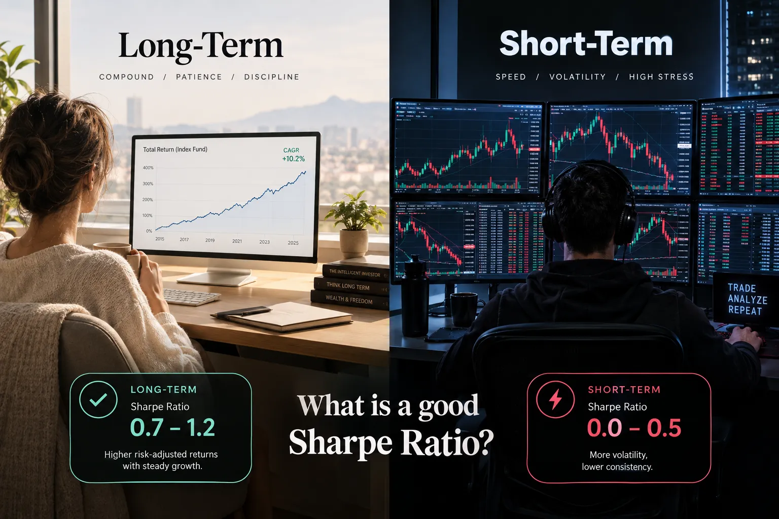
• Long-only stock or ETF portfolios. Measured over long periods, these tend to sit near the index. A good Sharpe ratio here is one that beats the index’s over the same window, after fees and taxes. Beating 0.43 by a little over decades is a real achievement.
• Swing trading bots. These hold for days to weeks and usually trade a small universe. Treat 1.0 or more, live and after costs, as good, and insist on several years of history because the trade count is modest.
• Day trading and intraday bots. More trades mean the estimate settles faster, but costs and slippage bite harder and returns are more likely to be serially correlated. Be extra careful with annualized daily figures, for the reasons Lo describes.
• Options-selling and grid bots. Expect flattering Sharpe ratios and look straight at the worst drawdown and the crash months. Our options backtesting guide explains why win rates and smooth curves mislead here.
• Market-neutral strategies. These remove most market exposure, so a modest Sharpe ratio can still mean real skill. Compare with other market-neutral approaches, not with the S&P 500.

Across all of them, the same three questions decide whether a number is a good Sharpe ratio or a lucky one: how long, how many variants, and what costs.

What Should You Check Besides the Sharpe Ratio?

No single ratio tells the whole story. Check a good Sharpe ratio alongside maximum drawdown, trade count, profit factor and out-of-sample results before you trust a bot with money.

• Maximum drawdown. The largest peak-to-trough loss. A 1.5 Sharpe ratio with a 60% drawdown is a different animal from a 1.5 with a 15% drawdown. This is what holding the strategy actually feels like.
• Trade count. A Sharpe ratio built on 40 trades is a guess; one built on thousands of trades across several market regimes is evidence.
• Profit factor. Gross profit divided by gross loss. It shows whether wins outweigh losses in dollars, which Sharpe does not show directly.
• Out-of-sample results. Performance on data the strategy never saw during development. Our coming guide to overfitting vs underfitting explains why this matters most.
• Costs and slippage. Model them at your real size and frequency. Free tools that do this honestly are compared in our best free backtesting software guide.
• How many variants were tried. The simulation above shows why this one question can matter more than the Sharpe ratio itself.

If you are building your own system, our coming quantitative trading guide walks through the full research loop. If you are comparing ready-made bots that advertise a good Sharpe ratio, see the automated AI trading bots directory and apply this checklist to every listing.

Decision rule: never fund a bot because it shows a good Sharpe ratio alone. Ask for drawdown, trade count, out-of-sample results and the number of variants tested as a package.

Frequently Asked Questions

What is a good Sharpe ratio?

A good Sharpe ratio is generally above 1.0, the level Investopedia describes as generally considered good. For a trading bot, judge it on live, cost-inclusive returns over several years. Treat anything above 3.0 as a claim to verify, because overfitting and short samples often inflate it.

Is a Sharpe ratio of 0.5 good?

Not for an active strategy or a paid bot. A 0.5 is below the 1.0 line, though it is close to the S&P 500’s long-run figure of about 0.43 on annual data since 1928. A bot should beat buy-and-hold on a risk-adjusted basis after costs to be worth paying for.

What is the Sharpe ratio of the S&P 500?

It depends on the window. On annual returns minus T-bills, it was about 0.43 from 1928 to 2025 and about 0.82 from 2015 to 2025, based on NYU Stern’s historical data. Trailing 12-month figures swing much more, from about 1.72 to 0.94 within 2026 on the sources we checked.

How do you calculate the Sharpe ratio?

Subtract the risk-free rate from each period’s return, average those excess returns, and divide by their standard deviation. Multiply a monthly figure by the square root of 12, or a daily figure by the square root of 252, to annualize. Check for autocorrelation first, because Lo found it can overstate annual Sharpe ratios by up to 65%.

Is a Sharpe ratio above 2 realistic for a trading bot?

It is possible but rare on a long live record, and common in backtests. In our simulation, the best of 100 strategies with zero real edge showed a Sharpe ratio of about 1.8 over two years. Ask how many variants were tested, how long the record is and whether costs are included.

Sharpe vs Sortino: which should I use?

Use both, then check drawdown. The Sortino ratio counts only downside deviation, so it is fairer to strategies with occasional big wins, but it can hide crash risk in strategies that collect small gains and rarely take large losses. Neither ratio replaces a look at the worst month.

How long a track record do I need to trust a Sharpe ratio?

Several years. In our simulation of a strategy with a true Sharpe ratio of 1.0, a one-year record showed zero or worse about 16% of the time, and a four-year record about 2% of the time. Short records tell you more through trade count and drawdown than through the Sharpe ratio.

Our Take

What is a good Sharpe ratio? Above 1.0, measured live, after costs, over a long enough record, and never trusted on its own. The index that built most retail wealth scored about 0.43 over nearly a century, which tells you how rare a real 2.0 is and how cheap a backtested one has become.

A bot with a boring, repeatable 1.2 over three years of live trading is worth more than a flashy 2.8 from a six-month backtest. Systems over hacks, every time. For more plain-English bot reviews and testing guides, start at AI Stock Trading Bots.

Have a bot with a live record worth checking? Send it to us and we will run the numbers.

Stay alpha.